Application - PlantLeaf

Audio Analysis Mode

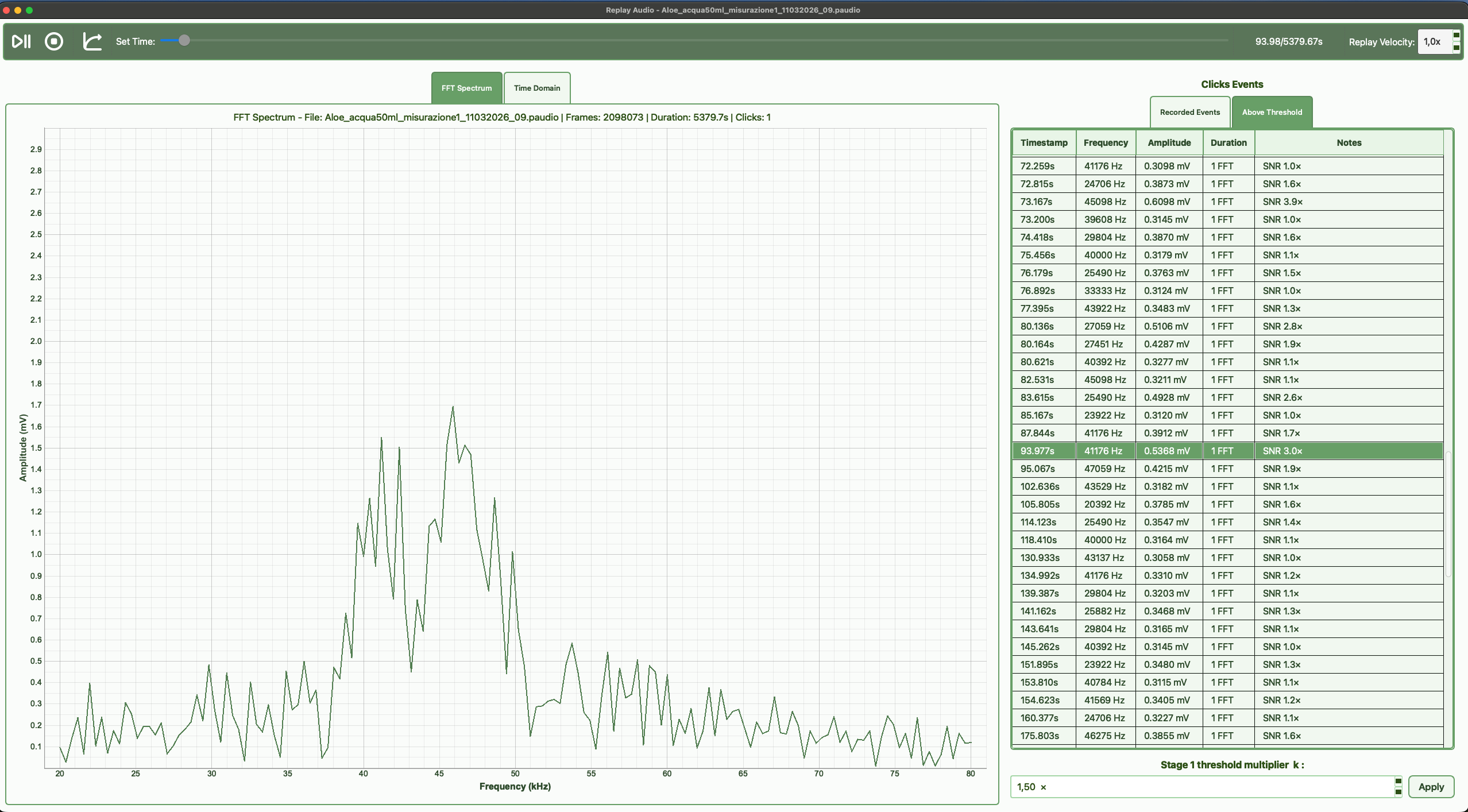
FFT Spectrum View

The main window displays the FFT spectrum of the current frame.

X-axis: frequency (20–80 kHz)
Y-axis: magnitude (volts)

A frame slider allows navigation through the recording. Playback controls can automatically advance frames. It is also possible to replay the recording at a slower rate to show every FFT frame.

Microphone Normalization

PlantLeaf compensates for the non-flat frequency response of the SPU0410LR5H-QB microphone using a conservative 50% correction (estimated error ±2.9 dB).

The correction is display-only and non-destructive, meaning the raw data in the file is never altered. But the corrected data is used by default for all downstream analysis, including the adaptive noise floor, event table and classifier.

Inverse FFT (iFFT)

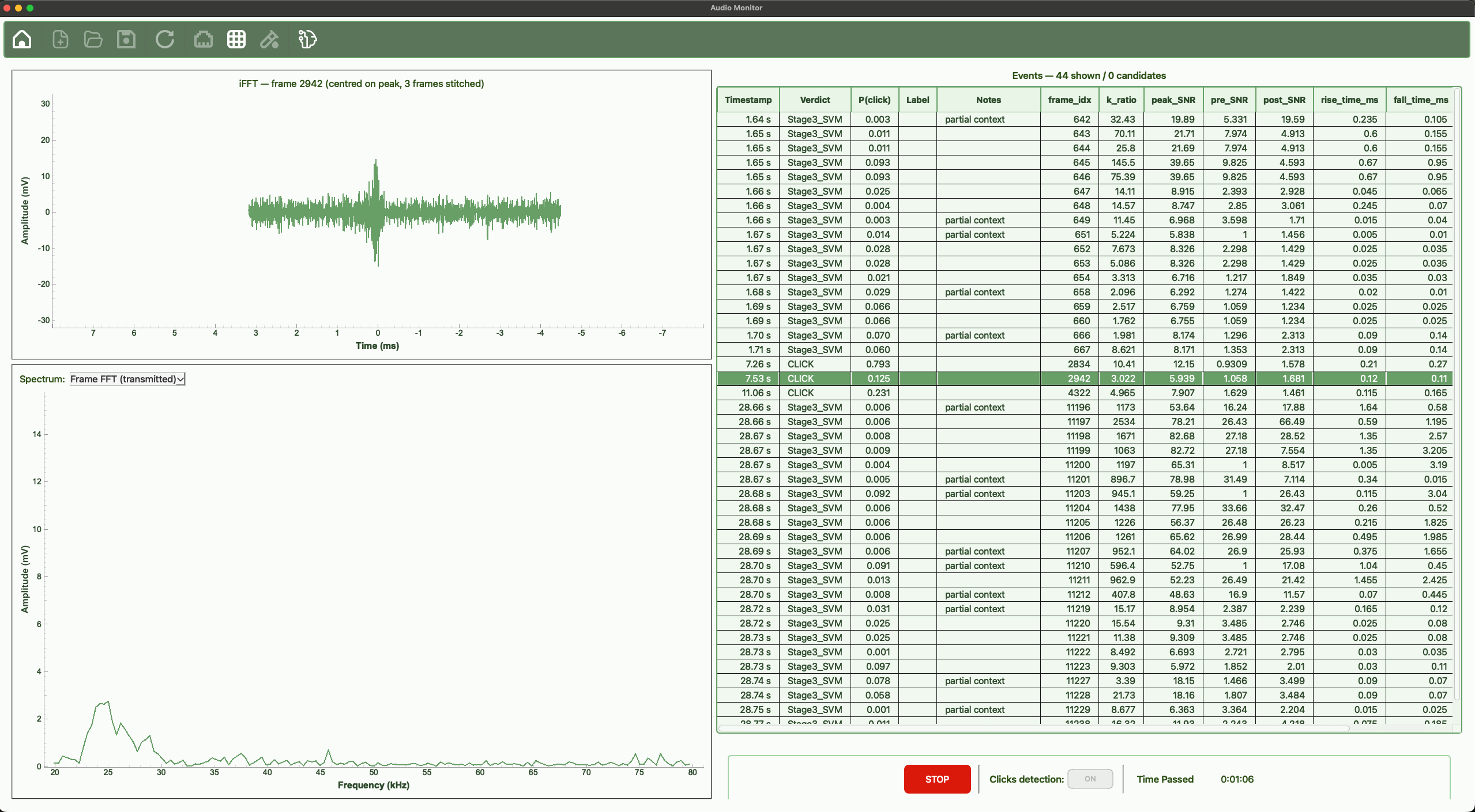
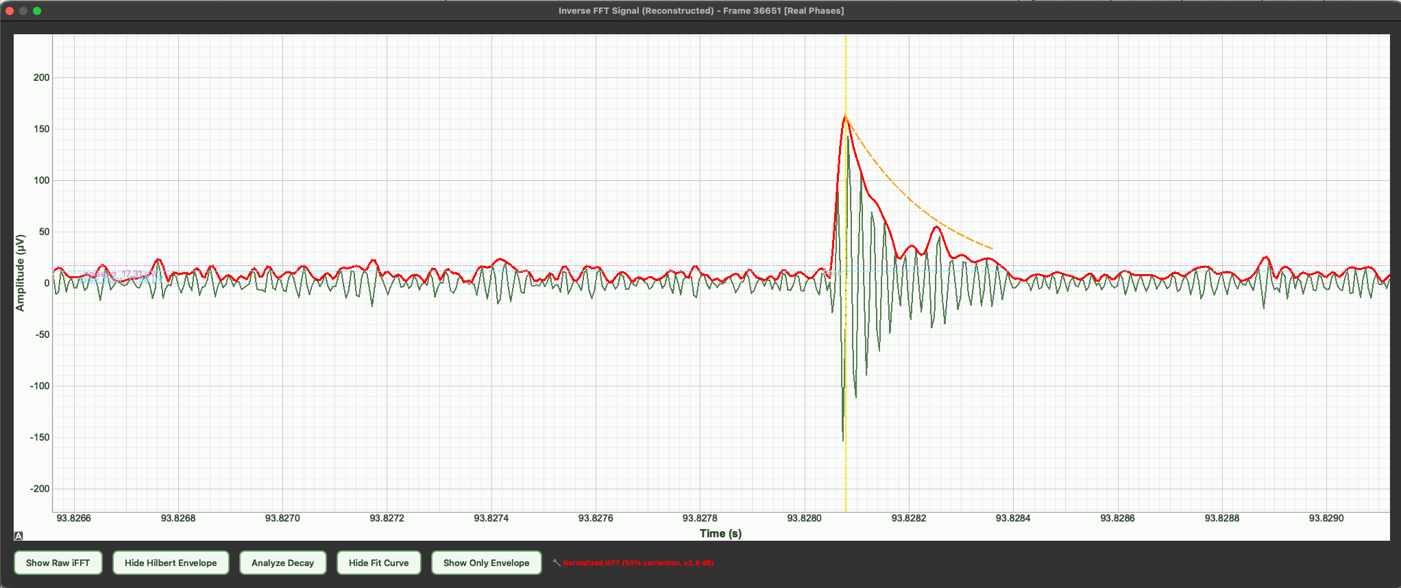
The iFFT tool reconstructs the time-domain waveform (512 samples) from FFT magnitude and phase data, applying a Tukey taper to suppress Gibbs ringing and allowing analysis with higher temporal resolution.

The window shows:

top panel: FFT spectrum
bottom panel: reconstructed waveform (512 samples)

Waveform characterization

Envelope and Decay Analysis

Additional tools are available for waveform characterization:

Hilbert Envelope – shows instantaneous amplitude over the reconstructed waveform.
Decay Analysis – fits the post-peak envelope to an exponential, extracting the decay constant τ, the fit quality R², and 17 physical features in total, each with an expected range for genuine clicks.

The exponential fit is overlaid on the envelope and colour-coded by fit quality — green (R² ≥ 0.70), orange (R² ≥ 0.45) and red (R² < 0.45) — helping to identify genuine ultrasonic click events at a glance.

Adaptive Analysis Tools

The app was rebuilt around an adaptive noise model so that the same tools work in silent rooms, noisy indoor spaces and outdoor environments — without manual recalibration.

Adaptive Noise Estimator

Instead of a single noise floor measured once per session, PlantLeaf tracks the floor in real time with a minimum-statistics estimator over a sliding window (~1.92 s). The estimate rises in noisy environments and falls in quiet ones, and is invariant to hardware gain — every downstream threshold and feature is derived from it.

Averaged Spectral View & Event Table

A time-averaged spectral view condenses long recordings into a single navigable overview. The event table then lists every candidate frame whose energy exceeds K × the adaptive noise floor (K is user-adjustable, range 0.5–20, default 1.5).

Mean FFT Window

Averaging the FFT across a window reveals the persistent spectral signature of a recording, separating steady background tones from the broadband, transient energy of genuine clicks.

Data Collection & Export

For every candidate, the app can export all 17 physical features to a CSV, alongside two-panel PNG snapshots (FFT spectrum + reconstructed waveform), ready for manual labelling. This is exactly the pipeline that produced the training set for our classifier — and the labelled dataset is available for download on the Database page.

Detection pipeline

Automatic Click Detection

The PlantLeaf app includes a 4-stage algorithm (version 5) that detects ultrasonic cavitation clicks in real time. Where earlier versions relied on fixed, hand-tuned thresholds that only worked in silent rooms, v5 replaces them with an adaptive noise floor and a trained machine-learning classifier — making it robust both indoors and outdoors, and across different hardware gains.

Adaptive energy threshold + run-length filter

Each 2.56 ms frame is scored by its average FFT energy and compared to k × the adaptive noise floor (k = 1.5). Because the floor is tracked in real time, the threshold rises in noisy environments and falls in quiet ones automatically. Runs of more than 3 consecutive above-threshold frames are discarded, since a genuine cavitation click cannot physically span that long.

Hard rejection gates

Two lenient gates discard events that are clearly not clicks before the expensive classification step. A frame is rejected if its exponential-decay fit fails (R² < 0.10) or if its Spectral Peak Ratio is extremely high (SPR ≥ 100) — the signature of a narrowband oscillator or electrical interference tone, completely unlike anything in the training data.

Feature extraction + SVM classification

Each surviving frame is reconstructed via inverse FFT and its Hilbert envelope computed. From this, 16 dimensionless features are extracted across three domains and fed to a trained classifier:

• Envelope — peak / pre / post SNR, rise & fall time, onset asymmetry, three zero-crossing rates, kurtosis.

• Decay fit — exponential time constant τ and its fit quality R².

• Spectrum — spectral peak ratio, low/high energy balance, dominant frequency, spectral-centroid shift.

An RBF support-vector machine (C = 50, γ = 0.01) makes the final decision. Its threshold is lowered to 0.220 to favour recall — missing a genuine click is costlier than a false positive a human can review. The most discriminative features are the fall time, peak SNR and dominant frequency.

Deduplication

When a click straddles two consecutive frames, only the frame with the higher peak amplitude is kept, eliminating any double counts.

Result

Trained on 285 labelled events (91 clicks + 194 hard-negative noise samples) from 38 sessions across 4 species, indoors and out, with a session-level split to prevent leakage. On a held-out test set the algorithm reaches recall 0.875, precision 0.824 and AUC 0.925 (cross-validated recall 0.907).

For full parameter details and the mathematical derivations, see the technical documentation on GitHub:

GitHub Documentation

Voltage mode

Voltage Curve-Fitting Analysis

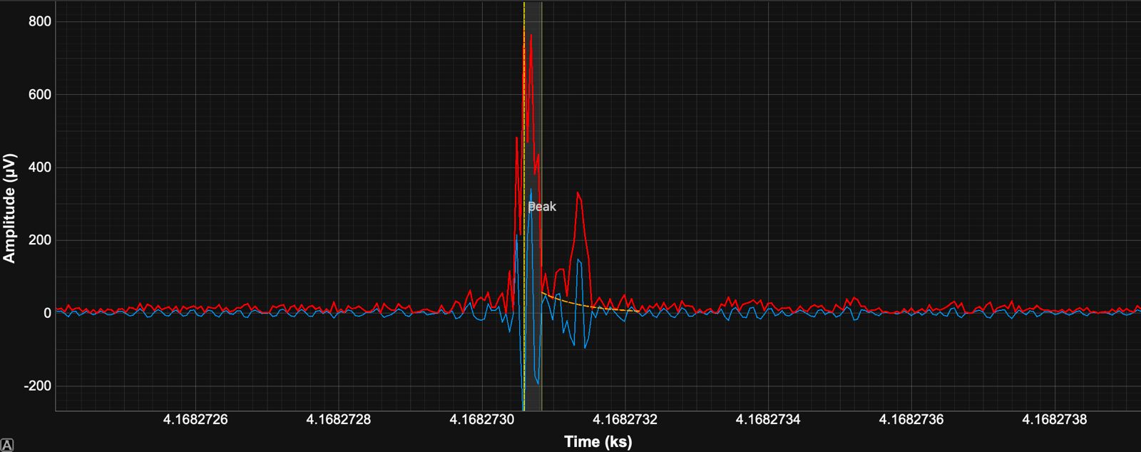
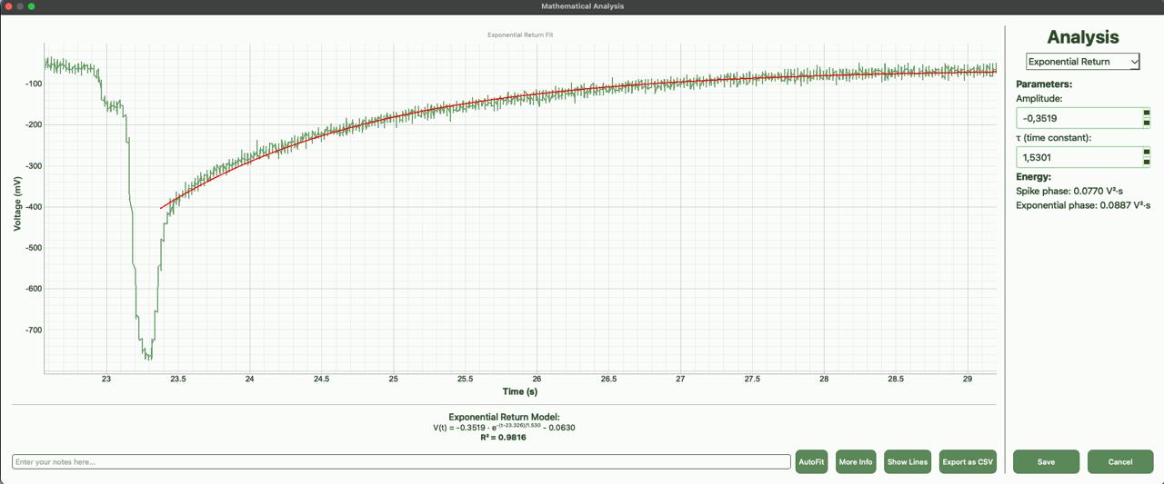
For electrical signals, the app automatically fits the best mathematical model to each selected event:

Exponential Return – a single decaying event.
Action Potential – a sinusoidal depolarisation followed by an exponential repolarisation, auto-detected when a rebound exceeds 30% of the main peak.

Fitting uses non-linear least squares scipy.optimize.curve_fit, reporting the goodness of fit R² in quality bands and the signal energy via trapezoidal integration. Across 20 recorded action potentials the model reached a mean R² of ≈ 0.976, confirming strong agreement with the observed physiology.