Audio

Ultrasonic Emission Detection

A recent study conducted by Tel Aviv University showed that stressed plants emit airborne ultrasonic sounds that can be heard from a distance. Thanks to their discoveries and our experiments we were able to identify features common to acoustic signals.

Frequency range
20–80 kHz
  • Most peaks between 40–80 kHz
  • The median peak frequency in our analysis was 42 kHz
Click duration
0.1–0.5 ms
  • Extremely short impulsive events
Sound pressure level
60–70 dB
  • Measured at 10 cm
  • Detectable at 3–5 m under controlled conditions
Event rate
Tens/hour
  • Healthy plants: very few clicks
  • Stressed plants: tens of events per hour
Biological origin of the signals

Biological origin of the signals

The emissions are thought to originate from xylem cavitation. During water transport, plants pull water upward through the xylem. Under stress (especially drought), increased tension can form and collapse air bubbles, generating microscopic mechanical vibrations. These vibrations propagate through plant tissue and into the air as ultrasonic clicks. While widely supported, the exact link between cavitation and airborne emissions is still under study.

Explore the acoustic simulator →
Leaf
What we know

What we know

What is clear from these studies and our experiments is that

Our study does have some limitations. Only a few plant species were tested, the experiments were conducted under semi-silent rooms and more data still needs to be collected. However, the results are promising and show that our instrumentation can effectively capture and analyze plant bioacoustic signals.

System overview

System overview

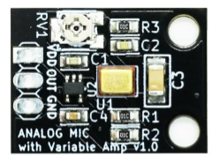
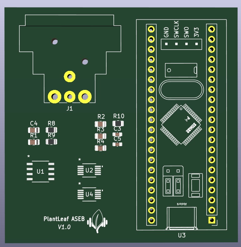
The ASEB board is the analog interface between the ultrasonic MEMS sensor and the digital acquisition system, conditioning weak ultrasonic signals before ADC conversion.

Main objectives

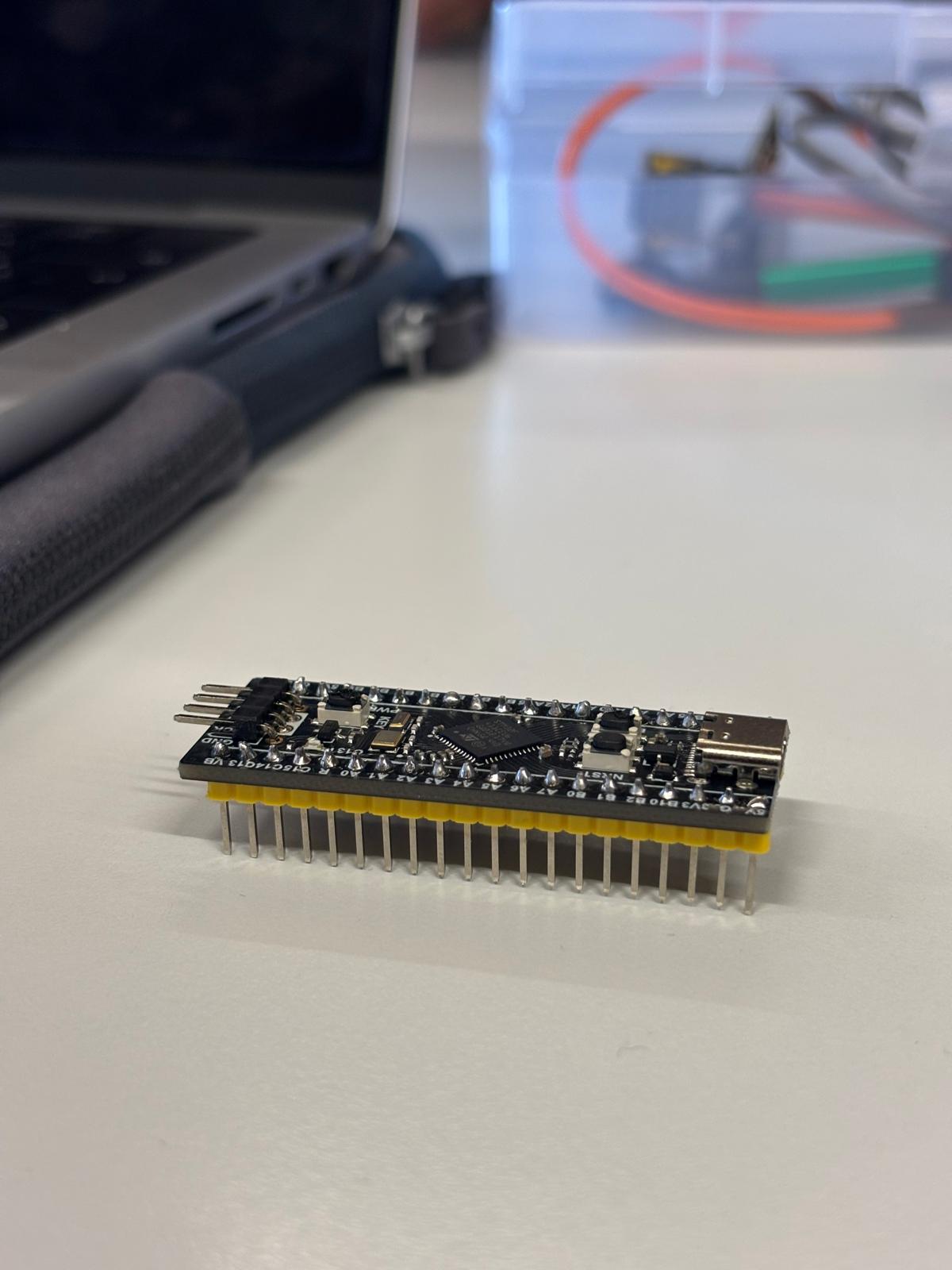
The analog chain consists of a dual OPA2365 active filtering stage followed by a fixed-gain OPA365 amplifier (~150×). The conditioned signal is then digitized by an STM32F411 microcontroller for further processing and analysis.

System overview
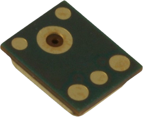
SPU0410LR5H-QB MEMS Microphone
Hardware architecture

Ultrasonic Microphone

The ASEB uses the SPU0410LR5H-QB MEMS microphone by Knowles as the primary sensing element. The sensor converts acoustic pressure variations into an analog electrical signal, allowing the detection of ultrasonic emissions potentially produced by plants.

More Information
System Architecture

The ASEB

The ASEB analog front-end is built around two main active components and dedicated RC filtering networks, providing low-noise signal conditioning, band limitation, and fixed amplification before the signal reaches the digital acquisition stage.

The current signal chain consists of

The previous variable-gain architecture has been removed in favor of a simpler and repeatable fixed-gain signal chain. All the technical documentation is available here.

Active Filtering
OPA2365

The first processing stage of the ASEB uses the OPA2365 dual operational amplifier to implement the active low-pass and high-pass filters.

  • Low noise, high bandwidth
  • Rail-to-rail input and output
  • 3.3 V single-supply operation
  • Low distortion

The two channels implement 2nd-order Sallen-Key low-pass and high-pass stages, at approximately unity gain, referenced to VREF = 1.65 V.

Fixed-Gain Amplification
OPA365 · ≈151×

After filtering, the signal is amplified by an OPA365 configured as a fixed-gain non-inverting amplifier.

  • Rf = 75 kΩ, Rg = 499 Ω
  • Fixed gain ≈ 151× (≈ 43.6 dB)

Gain applied after filtering avoids amplifying out-of-band signals. The old ADG704 configurable-gain stage is removed for a fixed, reproducible transfer function.

Analog Filtering
Sallen-Key, 20–80 kHz
  • High-pass, ≈ 12.9 kHz
  • Low-pass, ≈ 125.6 kHz

Filter frequencies sit outside the useful band, reducing attenuation and phase distortion in the 20–80 kHz measurement region.

Reduces environmental, mechanical, electronic and EMI noise before the OPA365 amplification stage.

Real Time Detection Firmware

Real Time Detection Firmware

The new v3 firmware moves the first stage of the detection algorithm onto the microcontroller itself. The device continuously measures its own noise floor, watches for the moment a frame rises above it, and transmits only those moments.

The analysis that used to happen hours later now happens as the click arrives: the waveform, the decay, and the classifier's verdict appear on screen while the plant is still being recorded.

Real Time Detection Firmware

From an applied perspective, this work aims to lay the foundations for a non-invasive, low-cost system capable of monitoring plant stress in real-world conditions. Such a tool could find applications in plant research, education, and potentially in precision agriculture, where early detection of stress could support more sustainable and targeted interventions. The emphasis on accessibility and scalability remains central, with the goal of making advanced plant monitoring techniques available beyond specialized laboratories, and all of this by starting from our own vegetable garden.

Microphone
Main characteristics
  • Type: Analog MEMS microphone
  • Frequency response: up to ~100 kHz
  • Output: analog voltage
  • Package: Surface-mount (SMD)
Advantages of MEMS microphones
  • Very small size
  • High manufacturing consistency
  • Low cost
  • Good sensitivity and stability

SPU0410LR5H-QB

The ASEB uses the SPU0410LR5H-QB MEMS microphone by Knowles as the primary sensing element. The sensor converts acoustic pressure variations into an analog electrical signal, allowing the detection of ultrasonic emissions potentially produced by plants.

Experiments

Audio Experiments

We have now accumulated roughly 160 hours of recordings across more than 150 sessions, grouped into three categories: ambient noise only, unstressed plants and stressed plants. We progressively moved from silent controlled rooms to noisier indoor environments and outdoor settings, annotating every session with the exact stress timing and any contaminating noise sources.

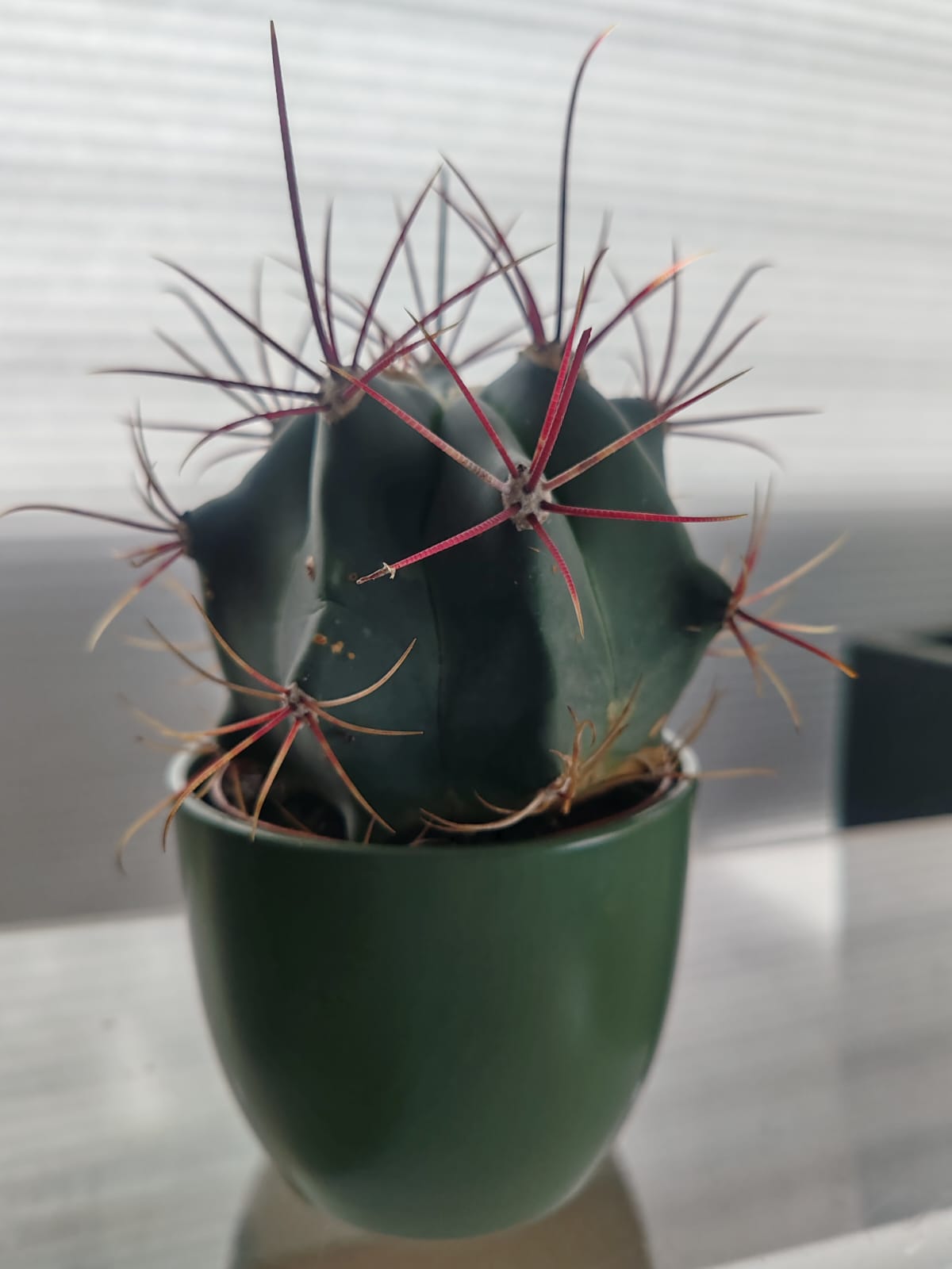
The analysis below covers the indoor part of that archive: 75 recordings, 74.5 hours — 22 with a stimulus applied during the recording (mechanical piercing of a leaf, or watering) against 53 controls (42 unstressed plants, 11 empty rooms). Six species are represented: Aloe vera, Ferocactus, Kalanchoe, Spathiphyllum, tomato and strawberry.

Clicks are counted in two independent ways. Automatically, by our detection algorithm (v6), on every recording; and by eye, on the 30 recordings a person reviewed event by event, judging each one from its spectrum and waveform. We report both, because an automatic count can only be trusted as far as someone has checked it — and every conclusion below holds under both.

Algorithm
Results

How many clicks

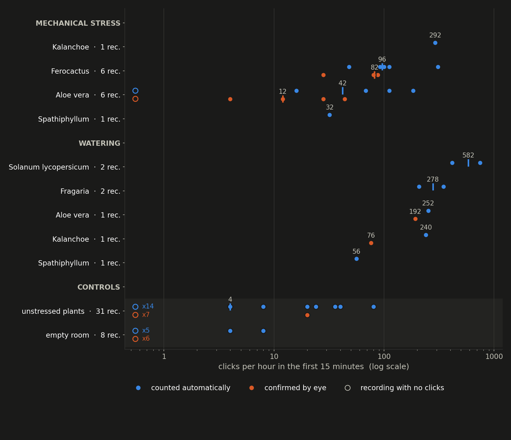
In the 15 minutes following a stimulus, mechanically stressed plants produced 105 clicks/hour counted automatically, and 41 clicks/hour counting only the ones confirmed by eye. Watered plants reached 324 and 134 clicks/hour. Unstressed plants stayed at 9.2 and 2.5, and empty rooms at 2.5 and 0.

Every rate is measured over the same 15 minutes of recording, so only recordings that run at least that long are included — 14 mechanically stressed, 7 watered, 31 unstressed and 8 empty-room. A recording that stops after a minute would turn three clicks into 170 per hour, which says more about its length than about the plant.

Compared against the unstressed plants' own first 15 minutes — the strictest control we have, since those recordings are handled at the start exactly like the others — mechanical stress raises the rate 11.5 times (95% confidence interval 8.9–15) and watering 35 times (28–46). Both windows are the first 15 minutes, on each side of the comparison.

Restricted to the recordings a person reviewed, and counting only the clicks they confirmed, the same window gives 16× for mechanical stress (95% confidence interval 6.8–52) and 54× for watering (22–170). Those intervals are wide because this comparison rests on far less material — 9 and 2 stressed recordings against 8 controls carrying 5 confirmed clicks in total — so we quote the automatic figures as the headline and these as the check that agrees with them.

By species under mechanical stress: Ferocactus 125 clicks/hour (6 recordings), Aloe vera 66 (6), Kalanchoe 292 (1) and Spathiphyllum 32 (1). After watering: tomato 582 (2 recordings), strawberry 278 (2), Aloe vera 252 (1), Kalanchoe 240 (1), Spathiphyllum 56 (1). The number of recordings behind each figure is shown beside it, because several species rest on a single session.

The clearest control result: across 7.3 hours of empty-room recording reviewed click by click, not a single click was confirmed.
Click rate per recording, by species, against both controls
Click rate in the first 15 minutes. One marker per recording, on a logarithmic scale; hollow markers are recordings with no clicks at all; the short bar is the group median.
Results

When they happen

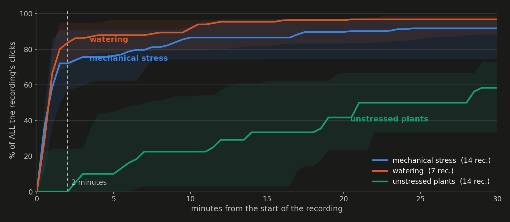
The response is immediate and short-lived. Of every click confirmed by eye in a mechanically stressed recording, 93% arrive within the first two minutes — and the stimulus itself is applied 30 to 60 seconds in. Counted automatically, which also picks up events a reviewer would reject, the share is 68% for mechanical stress and 78% for watering.

Unstressed plants show nothing of the kind. Only 27% of their clicks fall in the first two minutes, and 8 of the 14 unstressed recordings produce no click at all in that window — against 1 of 21 stressed recordings. Their emissions are spread across the whole session: half an hour in, the median unstressed recording has still delivered only 58% of its clicks, while a stressed one passed 70% before the two-minute mark.

Afterwards the plant falls quiet again: past the first 15 minutes, stressed recordings drop to about 0.4 confirmed clicks/hour — indistinguishable from an unstressed plant.

Cumulative arrival of clicks within a recording
Share of ALL the clicks in a recording that have arrived by a given minute — median across recordings, interquartile range shaded. A curve below 100% at the right edge means the rest of that recording's clicks come later.
Results

Detecting stress automatically

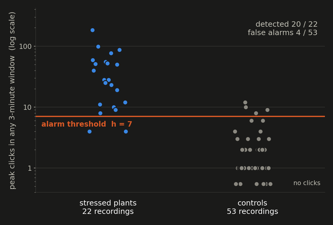
Counting clicks afterwards is one thing; raising an alarm while the plant is still emitting is another. Our detector keeps a sliding three-minute window over the incoming clicks and signals a stress event when the count crosses a threshold. That threshold is calibrated only on control recordings, chosen to tolerate at most 0.1 false alarms per hour, and never on the stressed recordings it is then tested against.

Tested one recording at a time, leaving that recording out of the calibration, it detects 20 of 22 stressed recordings and raises 4 false alarms in 44.7 hours of control recording (0.09 per hour; 95% upper bound 0.21). The separation between stressed and control recordings corresponds to an area under the ROC curve of 0.98, and the calibrated threshold came out identical in every single fold. The two misses are quiet Aloe recordings with 5 and 7 clicks in total, which no threshold would catch.

Automatic stress detection against its calibrated threshold
Peak number of clicks in any three-minute window, one marker per recording, against the alarm threshold calibrated on control recordings alone.
Honesty

What we do not claim

These results are indoor only. Outdoors, environmental sounds recorded with no plant present produce more detections than recordings of plants do, so our algorithm is not yet reliable in that setting and we report no outdoor rates.

A burst of environmental false positives is, to a burst detector, indistinguishable from a burst of plant clicks. This is a property of the method, not a bug to be tuned away, and it is why a person reviewed a third of the recordings by hand.

While analysing the corpus we found a narrowband 66 kHz interference tone contaminating nine recordings — a fixed, low-amplitude line, unlike the broadband clicks of a plant. Those recordings are identified and excluded before any number above is computed. Finally, the classifier was trained on part of this material, so the automatic counts on those recordings are optimistic; the counts confirmed by eye are not.

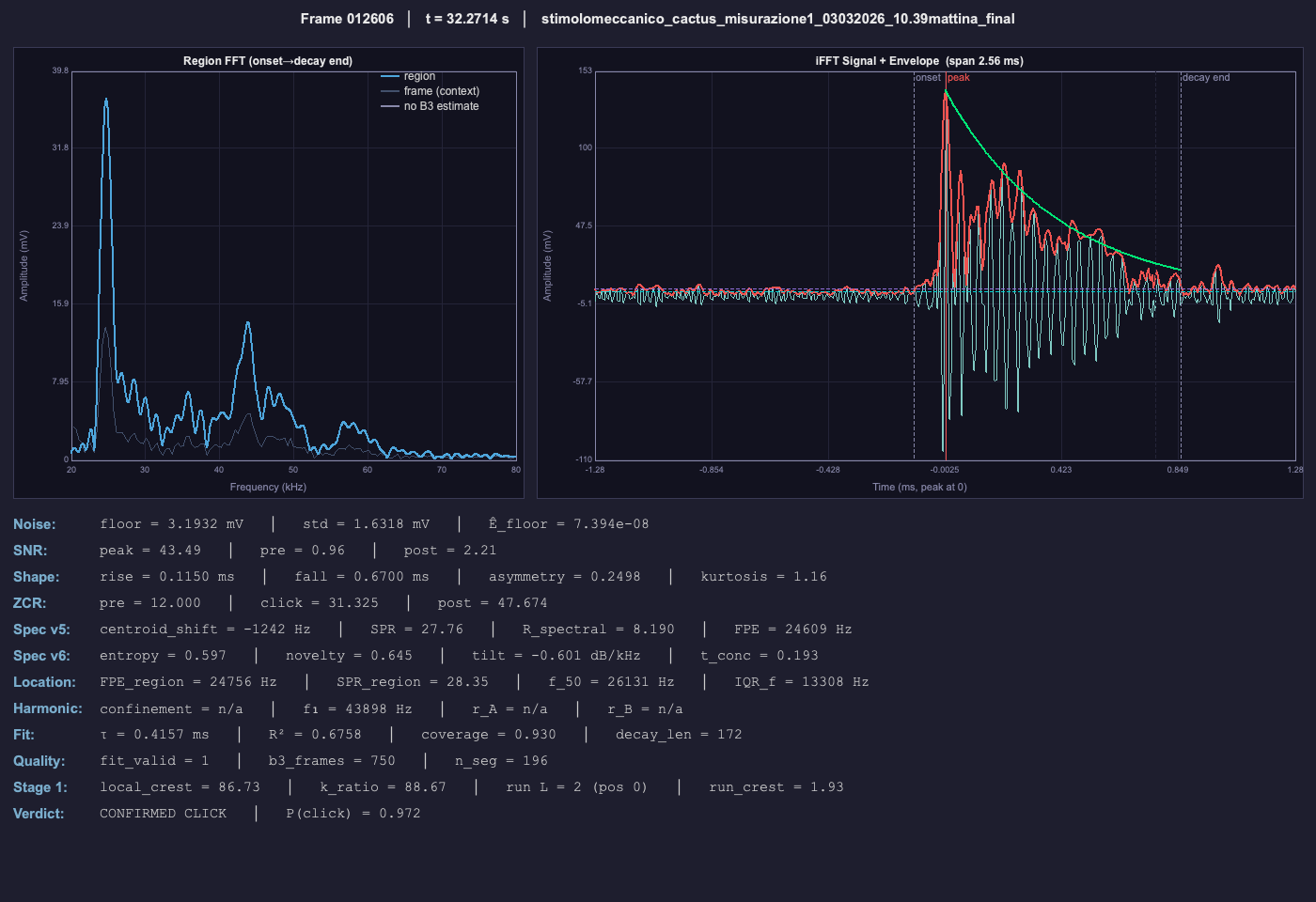
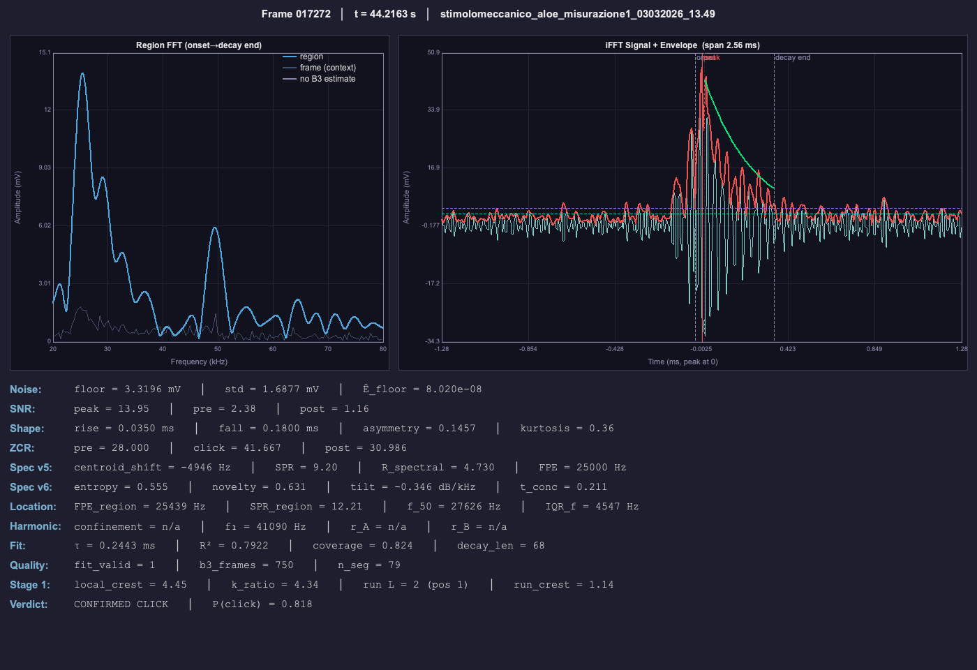
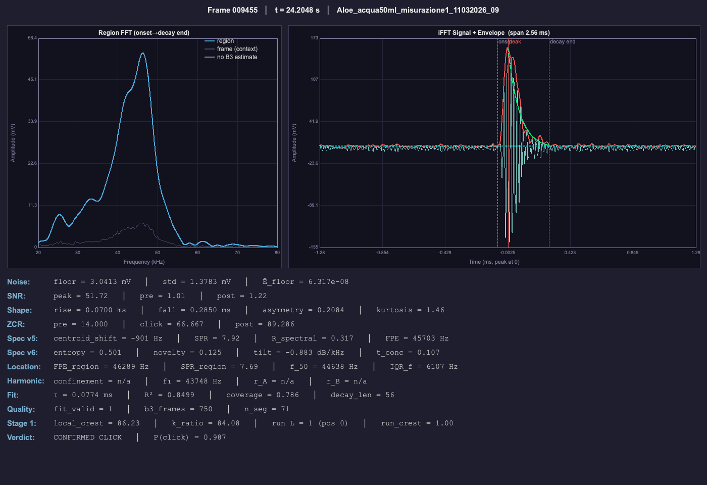
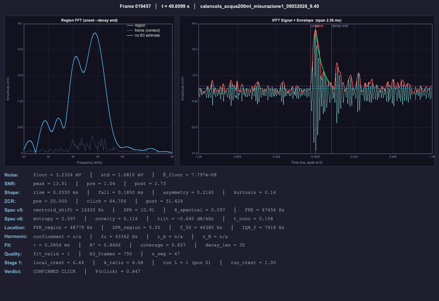
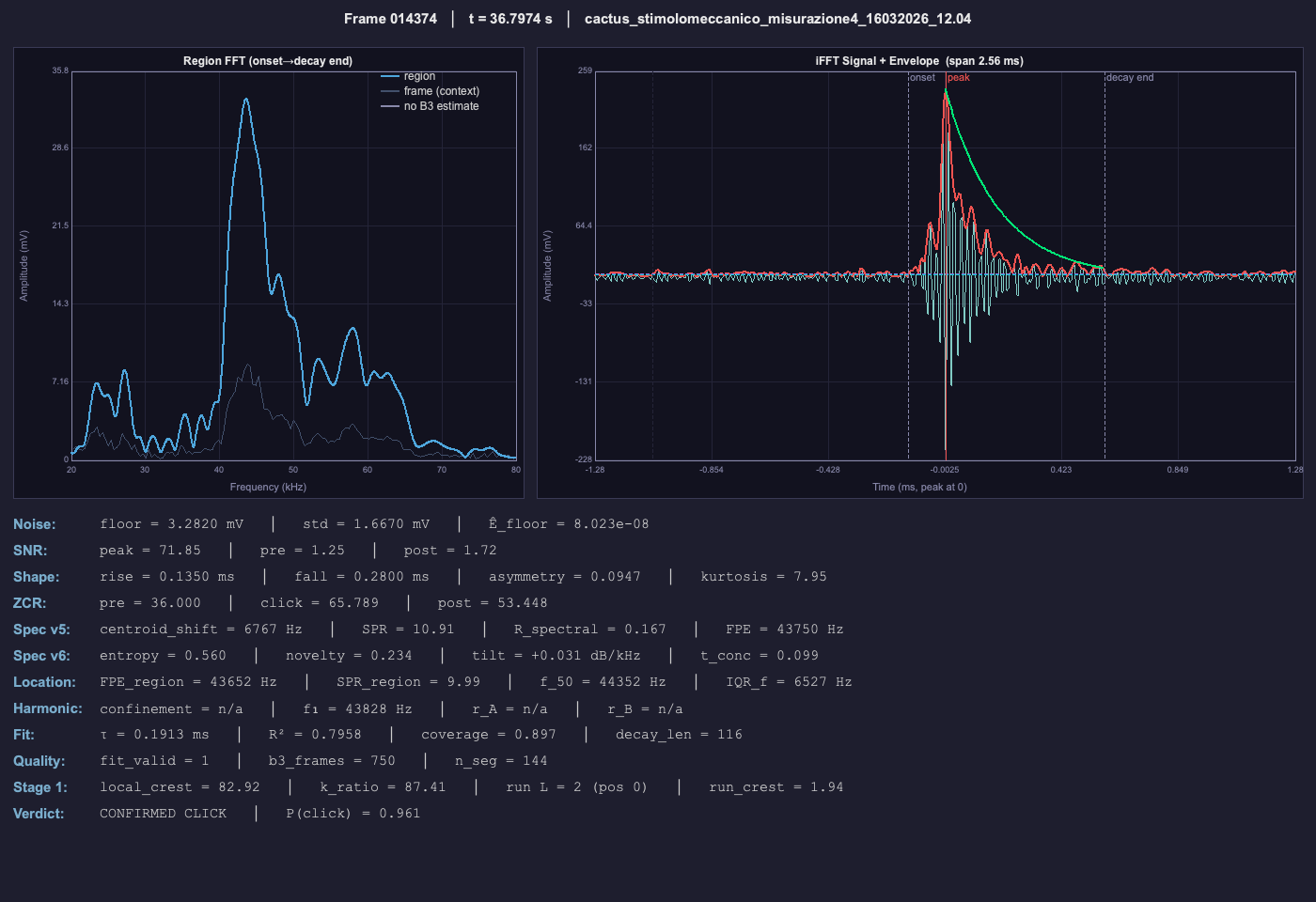
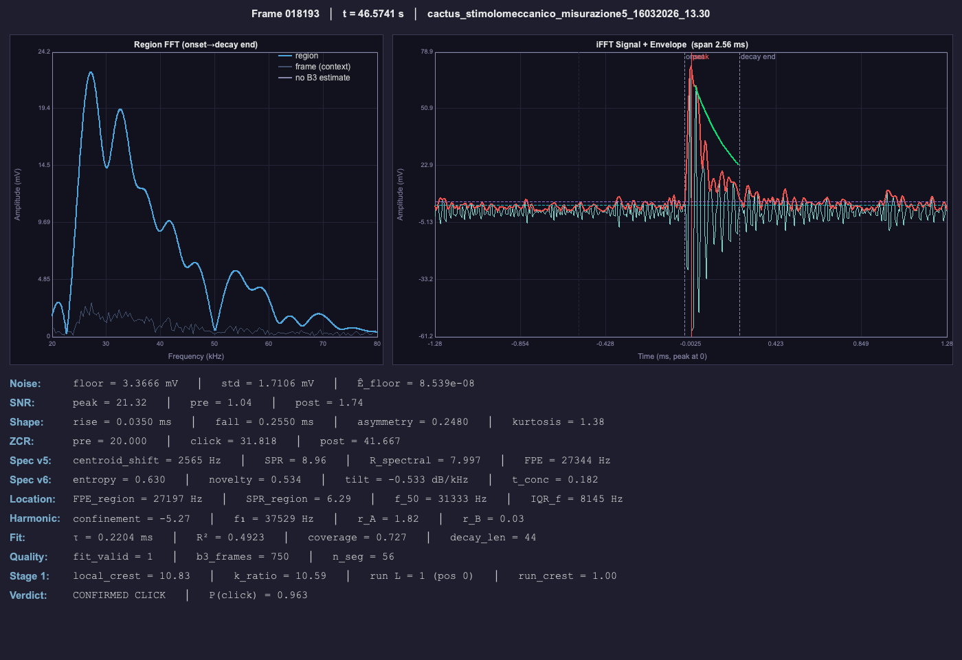
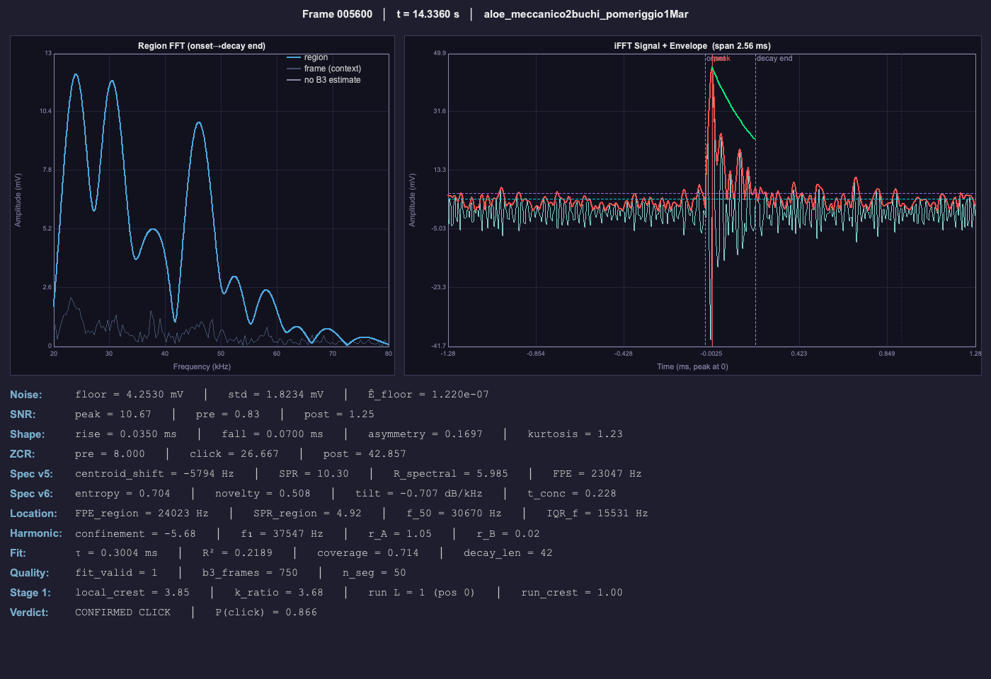
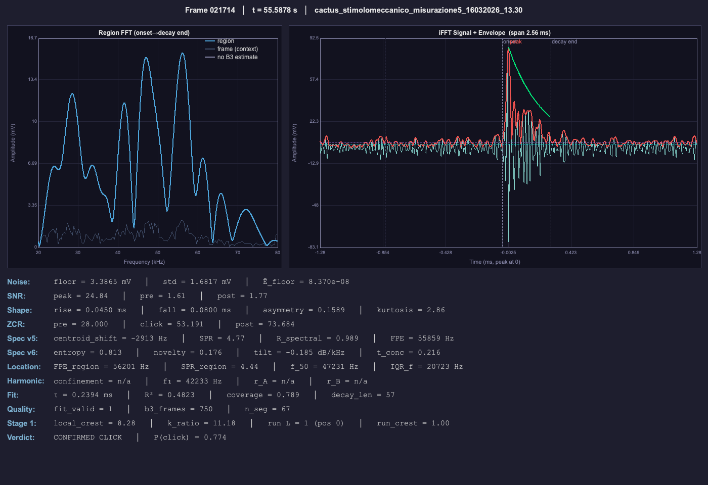
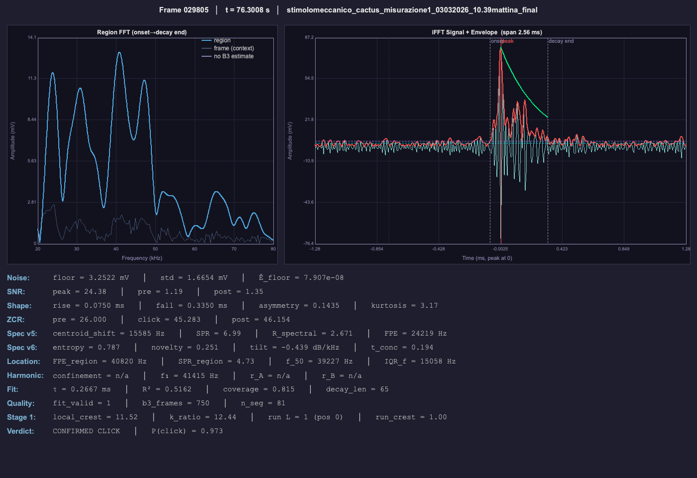
Nine clicks from our recordings, each one confirmed by eye and then measured by the v6 algorithm. The left panel is the spectrum of the click itself against the surrounding frame; the right panel is the waveform reconstructed by inverse FFT, with its amplitude envelope and the fitted exponential decay. Every measured parameter is printed under the plots — click any image to read them, ending with P(click), the probability the classifier assigns to it being a genuine cavitation click.

Ferocactus, mechanical stress, P(click) 0.97
Ferocactus — mechanical stress
SNR 43.5 · τ 0.42 ms · R² 0.68 · 24.6 kHz · P(click) 0.97
Aloe vera, mechanical stress, P(click) 0.82
Aloe vera — mechanical stress
SNR 13.9 · τ 0.24 ms · R² 0.80 · 25.0 kHz · P(click) 0.82
Aloe vera, after watering, P(click) 0.99
Aloe vera — after watering
SNR 51.7 · τ 0.08 ms · R² 0.85 · 45.7 kHz · P(click) 0.99
Kalanchoe, after watering, P(click) 0.85
Kalanchoe — after watering
SNR 13.5 · τ 0.09 ms · R² 0.87 · 47.7 kHz · P(click) 0.85
Ferocactus, mechanical stress, P(click) 0.96
Ferocactus — mechanical stress
SNR 71.8 · τ 0.19 ms · R² 0.80 · 43.8 kHz · P(click) 0.96
Ferocactus, mechanical stress, P(click) 0.96
Ferocactus — mechanical stress
SNR 21.3 · τ 0.22 ms · R² 0.49 · 27.3 kHz · P(click) 0.96
Aloe vera, mechanical stress, P(click) 0.87
Aloe vera — mechanical stress
SNR 10.7 · τ 0.30 ms · R² 0.22 · 23.0 kHz · P(click) 0.87
Ferocactus, mechanical stress, P(click) 0.77
Ferocactus — mechanical stress
SNR 24.8 · τ 0.24 ms · R² 0.48 · 55.9 kHz · P(click) 0.77
Ferocactus, mechanical stress, P(click) 0.97
Ferocactus — mechanical stress
SNR 24.4 · τ 0.27 ms · R² 0.51 · 40.1 kHz · P(click) 0.97

Method

Method for Recording and Analysis

Finding a method to reliably spot ultrasonic clicks generated by plants played a crucial role. We collected three categories of recordings: only ambient noise, unstressed plants and stressed plants. Starting from silent, controlled rooms, we progressively shifted toward noisier indoor environments and eventually outdoor settings. In total, we accumulated approximately 160 hours of recordings across over 150 sessions, each annotated with the exact timing of stress events and any noise sources that could have contaminated the recording. Careful analysis initially consisted of comparing potential clicks with those of Khait et al. and examining their most consistent characteristics: broadband FFT spectra and iFFTs resembling damped sine waves lasting 0.1–0.5 ms. As confirmed clicks accumulated, we began extracting physical features to describe them quantitatively. This process, eventually, led to the development of the automatic Click Detection Algorithm.

Algorithm